Diffusion coefficient and viscosity

The diffusion coefficient  of a Zimm chain can be easily calculated from Eqs. (7.16) and (7.17). The result is

$$\frac{kT}{2}\frac{\mu _{00}}{N+1}=\frac{kT}{6\pi \eta b}\sqrt{\fr... ...} \frac{1}{(N+1)^{2}}\sum_{n=0}^{N}\sum_{m=0}^{N}\frac{1}{\vert n-m\vert^{1/2}}$$ D_G = (7.19)

$$\approx \frac{kT}{6\pi \eta b}\sqrt{\frac{6}{\pi }}\frac{1}{N^{2}} \int_{0}^{N}dn\int_{0}^{N}dm\frac{1}{\vert n-m\vert^{1/2}}$$ (7.20)

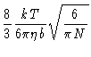$$\frac{8}{3}\frac{kT}{6\pi \eta b}\sqrt{\frac{6}{\pi N}}$$ = (7.21)

The diffusion coefficient now scales with N^-1/2, in agreement with experiments.

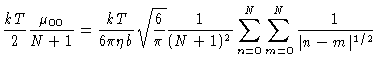
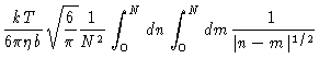
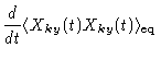
In order to calculate the intrinsic viscosity  of a dilute solution of Zimm chains we go back to Eq. (6.64):

$$\frac{d}{dt}\langle X_{kx}(t)X_{ky}(t)\rangle =-\frac{2}{\tau... ..._{ky}(t)\rangle +\dot{\gamma}\langle X_{ky}(t)X_{ky}(t)\rangle$$ (7.22)

Again we shall approximate $\langle X_{ky}(t)X_{ky}(t)\rangle$ by its equilibrium value. At the end of this section we shall show that

$$\langle X_{ky}X_{ky}\rangle _{\mathrm{eq}}=kT\frac{\mu _{kk}}{N+1}\frac{\tau _{k}}{2}$$ (7.23)

The solution of Eq. (7.22) with this approximation is

$$\langle X_{kx}(t)X_{ky}(t)\rangle =kT\frac{\mu _{kk}}{N+1}\le... ...rac{\tau _{k}}{2}\right) ^{2}(1-e^{-2t/\tau _{k}})\dot{\gamma}$$ (7.24)

Eqs. (6.53), (6.57) and (7.24) then yield

$$\lbrack \eta ]=\frac{N_{Av}}{M}12\pi \left\{ \frac{(N+1)b^{2}}{12\pi } \right\} ^{3/2}\sum_{k=1}^{N}\frac{1}{k^{\frac{3}{2}}}$$ (7.25)

The intrinsic viscosity scales with N^3/2, in agreement with experiments.

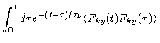
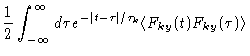
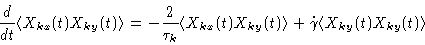
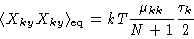
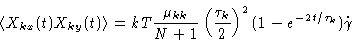
We finish this section by proving Eq. (7.23). At equilibrium we have

 

$$\frac{d}{dt} \langle X_{ky}(t) X_{ky}(t) \rangle_{\mathrm{eq}}$$ 0 = (7.26)

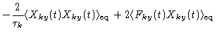$$-\frac{2}{\tau_k} \langle X_{ky}(t) X_{ky}(t) \rangle_{\mathrm{eq}} + 2 \langle F_{ky}(t) X_{ky}(t) \rangle_{\mathrm{eq}}$$ = (7.27)

The last term here can be calculated according to

 

$$\langle F_{ky}(t) X_{ky}(t) \rangle \int_0^t d\tau e^{-(t-\tau)/\tau_k} \langle F_{ky}(t) F_{ky}(\tau) \rangle$$ = (7.28)

$$\frac{1}{2} \int_{-\infty}^{\infty} d\tau e^{-\vert t-\tau\vert/\tau_k} \langle F_{ky}(t) F_{ky}(\tau) \rangle$$ = (7.29)

Eq. (7.27), (7.29) and (7.17) yield Eq. ( 7.23).