We now apply the RISM formalism to polymeric liquids . For simplicity we restrict the presentation to
polyethylene , each
CH2 will be viewed as one ''atom''.
It is clear that if boundary effects may be neglected, all monomers along
the chain are equivalent, i.e. that
![]() and all other
functions do not depend on
and all other
functions do not depend on ![]() or
or ![]() .
Remember that
.
Remember that ![]() and
and ![]() each run from 0 to N, where (N+1) is the number of
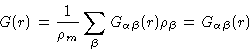
monomers per chain. The monomer-monomer radial distribution function then is
each run from 0 to N, where (N+1) is the number of
monomers per chain. The monomer-monomer radial distribution function then is
| (2.38) |
We now apply the method to polyethylene, which will be modelled by a RIS
model with characteristics given in section 2.6. The interaction between two
monomers on different chains is modelled by a hard sphere interaction with
diameter
![]() .
Moreover N=6416 and
.
Moreover N=6416 and
![]() .
Calculations were done with PY closure.
.
Calculations were done with PY closure.
In Fig. (2.3) is given the intermolecular distribution function. We clearly see what is called the ''correlation hole'' by de Gennes ; the intermolecular distribution gradually rises to its limit value 1, with only little structure. The scattering function is given in Fig. (2.4), and is in perfect agreement with X-ray experiments, except at very small values of k.
We give two more results, from MD simulations this time. In Fig. (2.5
) is given the intramolecular oxygen-oxygen correlation in PEO . The simulation was done with GROMOS united atom
potentials. The box consisted of two chains of 800 monomers each;
![]() and T=400K. The corresponding intermolecular
correlation function is given in Fig. (2.6).
and T=400K. The corresponding intermolecular
correlation function is given in Fig. (2.6).

![\scalebox{0.5}{\includegraphics[14,85][580,385]{fig2_3.eps}}](img241.gif)
![\scalebox{0.5}{\includegraphics[14,85][580,385]{fig2_4.eps}}](img242.gif)
![\scalebox{0.5}{\includegraphics[14,450][580,760]{fig2_5.eps}}](img243.gif)
![\scalebox{0.5}{\includegraphics[14,450][580,760]{fig2_6.eps}}](img244.gif)