Green's function method

In this section we shall investigate the Gaussian chain  at a level where the distance between two consecutive beads may be considered to be small.

Suppose we study a Gaussian chain in an external field  with potential $\Phi ( \vec{R})$. The distribution in configuration space then reads

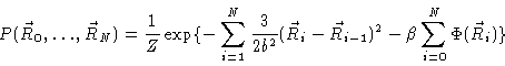$$P(\vec{R}_{0},\ldots ,\vec{R}_{N})=\frac{1}{Z}\exp \{-\sum_{i... ...}-\vec{R}_{i-1})^{2}-\beta \sum_{i=0}^{N}\Phi (\vec{R} _{i})\}$$ (3.12)

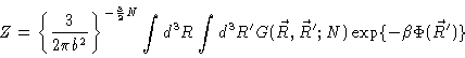
where Z is a normalizing constant. In many cases we are interested in properties depending on the position vectors of only a few beads along the chain. It will turn out to be useful then to introduce the Green's function 

 

$${G(\vec{R},\vec{R}\prime ;N)=\left\{ \frac{3}{2\pi b^{2}}\right\} ^{\frac{3}{2}N}\int d^{3}R_{1}\ldots \int d^{3}R_{N-1}}$$

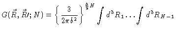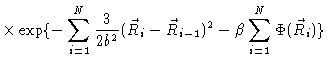$$\times \exp \{-\sum_{i=1}^{N}\frac{3}{2b^{2}}(\vec{R}_{i}-\vec{R} _{i-1})^{2}-\beta \sum_{i=1}^{N}\Phi (\vec{R}_{i})\}$$ (3.13)

where $\vec{R}_{0}=\vec{R}^{\prime }$ and $\vec{R}_{N}=\vec{R}$. Notice that the Green's function is not normalized. One easily verifies however

$$G(\vec{R},\vec{R}^{\prime };N+n)=\int d^{3}R^{\prime \prime }... ...me \prime };n)G(\vec{R}^{\prime \prime },\vec{R}^{\prime };N).$$ (3.14)

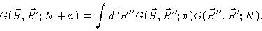
This equation is called the Chapman-Kolmogorov equation . For this equation to hold true, it is essential that the second summation in the exponent in Eq. (3.13) starts at i=1, and not at i=0 as in Eq. (3.12).

Now we shall treat N like a continuous variable. In Appendix C we shall prove that $G( \vec{R},\vec{R}^{\prime};N)$ is the solution of

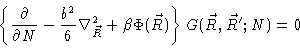$$\left\{ \frac{\partial}{\partial N} - \frac{b^2}{6} \nabla_{\... ...beta \Phi (\vec{R}) \right\} G(\vec{R},\vec{R}^{\prime};N) = 0$$ (3.15)

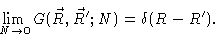$$\lim_{N \rightarrow 0} G(\vec{R},\vec{R}^{\prime};N) = \delta (R-R^{\prime}) .$$ (3.16)

Accepting this for the moment we may immediately write down the formal solution

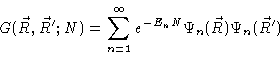$$G(\vec{R},\vec{R}^{\prime};N) = \sum_{n=1}^{\infty} e^{-E_n N} \Psi_n ( \vec{R}) \Psi_n (\vec{R}^{\prime})$$ (3.17)

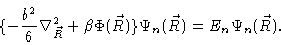$$\{ - \frac{b^2}{6} \nabla_{\vec{R}}^2 + \beta\Phi (\vec{R}) \} \Psi_n (\vec{R })= E_n \Psi_n (\vec{R}) .$$ (3.18)

One easily checks this by introducing Eq. (3.17) into Eq. ( 3.15) and using Eq. (3.18). Eq. (3.16) is nothing but the closure equation of the complete set of functions.

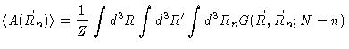
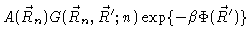
Knowing $G( \vec{R},\vec{R}^{\prime};N)$ makes it possible to calculate all kinds of averages:

$$Z = \left\{ \frac{3}{2\pi b^2} \right\}^{-\frac{3}{2}N} \int ... ...,\vec{R}^{\prime};N) \exp\{- \beta \Phi (\vec{R} ^{\prime}) \}$$ (3.19)

$${ \langle A(\vec{R}_n) \rangle = \frac{1}{Z} \int d^3R \int d^3R' \int d^3R_n G(\vec{R},\vec{R}_n;N-n) }$$

$$A(\vec{R}_n) G(\vec{R}_n,\vec{R}^{\prime};n) \exp\{- \beta\Phi (\vec{R} ^{\prime}) \}$$ (3.20)

etc.