B. The stress tensor in normal coordinates

The beads in our polymer are assumed to be point particles. The second term in Eq. (5.64) is proportional to the volume fraction of beads, and therefore equals zero. The element S_xy(t) of the stress tensor  then reads

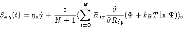$$S_{xy}(t)=\eta _{\mathrm{s}} \dot{\gamma}+\frac{\mathrm{c}}{N... ...}{\partial R_{iy}}(\Phi +k_{B}T\ln \Psi )\rangle _{\mathrm{c}}$$ (6.54)

where c is the monomer concentration. The $\ln \Psi$ term yields

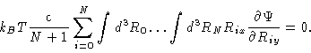$$k_{B}T\frac{\mathrm{c}}{N+1}\sum_{i=0}^{N}\int d^{3}R_{0}\ldots \int d^{3}R_{N}R_{ix}\frac{\partial \Psi }{\partial R_{iy}}=0.$$ (6.55)

So, we are left with

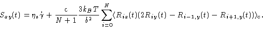$$S_{xy}(t)=\eta _{\mathrm{s}}\dot{\gamma}+\frac{\mathrm{c}}{N+... ...t)(2R_{iy}(t)-R_{i-1,y}(t)-R_{i+1,y}(t))\rangle _{\mathrm{c}}.$$ (6.56)

We next introduce the normal mode expansion Eq. (6.24), and go through the usual analysis; finding

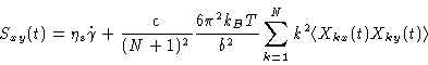$$S_{xy}(t)=\eta _{\mathrm{s}}\dot{\gamma}+\frac{\mathrm{c}}{(N... ...}T}{b^{2}}\sum_{k=1}^{N}k^{2}\langle X_{kx}(t)X_{ky}(t)\rangle$$ (6.57)

From now on we omit the subscript c at the averaging brackets, because it serves no purpose anymore.