The mean square end-to-end vector

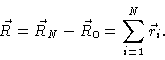
A rough measure of the average size of the polymer is given by the mean square end-to-end vector , which we shall calculate in this section. Related properties are the radius of gyration , and the persistence length . Both of them may be calculated using methods similar to the ones in this section.

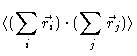
The end-to-end vector is given by

$$\vec{R} = \vec{R}_N - \vec{R}_0 = \sum_{i=1}^N \vec{r}_i.$$ (1.27)

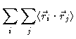
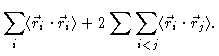
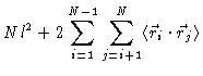
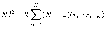
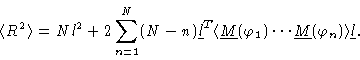
The mean square then reads

$$\langle R^2 \rangle \langle (\sum_i \vec{r}_i) \cdot (\sum_j \vec{r} _j) \rangle$$ =

$$\sum_i \sum_j \langle \vec{r}_i\cdot\vec{r}_j \rangle$$ =

$$\sum_i \langle \vec{r}_i\cdot\vec{r}_i \rangle + 2 \sum \sum_{ i<j} \langle \vec{r}_i\cdot\vec{r}_j\rangle .$$ = (1.28)

Again assuming the chain is infinitely long, we may put $\langle \vec{r}_i \cdot \vec{r}_{i+n} \rangle$ independent on i. Then

 

$$\langle R^2 \rangle Nl^2 + 2 \sum_{i=1}^{N-1} \sum_{j=i+1}^{N} \langle \vec{r}_i \cdot \vec{r}_j \rangle$$ =

$$Nl^2 + 2 \sum_{n=1}^N (N-n) \langle \vec{r}_i \cdot \vec{r} _{i+n}\rangle$$ = (1.29)

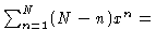
where (N-n) is the number of times the distance n may occur along the chain.

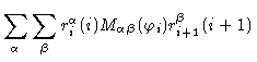
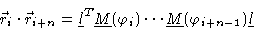
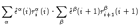
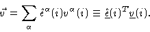
We now set forth to calculate $\langle \vec{r}_i \cdot \vec{r}_{i+n} \rangle$. In order to do so we need to calculate the scalar product $\vec{r}_i \cdot \vec{r}_{i+n}$ as a function of the angles $\varphi_i,\ldots, \varphi_{i+n-1}$. To this end we associate with every monomer i a Cartesian coordinate system $\hat{e}^{\alpha}(i)$. Every vector $\vec{v}$may then be expanded like

$$\vec{v} = \sum_{\alpha} \hat{e}^{\alpha}(i) v^{\alpha}(i) \equiv \underline{ \hat{e}}(i)^T \underline{v}(i).$$ (1.30)

The precise definition of the local coordinate system is given in Appendix A. Here we only mention that

$$\vec{r}_i l \hat{e}^3(i)$$ =

$$\underline{r}_i l(0,0,1)^T \equiv \underline{l} .$$ = (1.31)

A particular example of Eq. (1.30) is

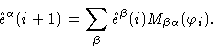$$\hat{e}^{\alpha} (i+1) = \sum_{\beta} \hat{e}^{\beta}(i) M_{\beta\alpha}(\varphi_i) .$$ (1.32)

The matrix $\underline{M}(\varphi)$ is calculated in Appendix B.

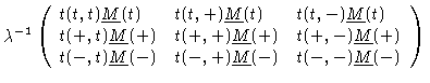
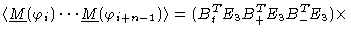
The scalar product $\vec{r}_i \cdot \vec{r}_{i+1}$ now reads

$$\vec{r}_i \cdot \vec{r}_{i+1} \sum_{\alpha} \hat{e}^{\alpha}(i) r_i^{\alpha}(i) \cdot \sum_{\beta} \hat{e}^{\beta} (i+1) r_{i+1}^{\beta} (i+1)$$ =

$$\sum_{\alpha} \sum_{\beta} r_i^{\alpha}(i) M_{\alpha\beta}(\varphi_i) r_{i+1}^{\beta}(i+1)$$ =

$$\underline{l}^T \underline{M}(\varphi_i) \underline{l}$$ = (1.33)

and in general

$$\vec{r}_i \cdot \vec{r}_{i+n} = \underline{l}^T \underline{M}(\varphi_i) \cdots \underline{M}(\varphi_{i+n-1}) \underline{l}$$ (1.34)

from which we get

$$\langle R^2 \rangle = N l^2 + 2 \sum_{n=1}^N (N-n) \underline... ...phi_1) \cdots \underline{M}(\varphi_n) \rangle \underline{l }.$$ (1.35)

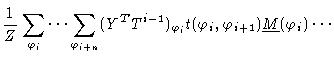
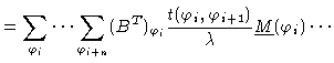
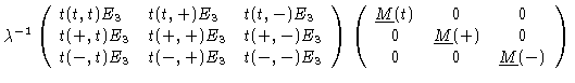
We finally calculate the remaining average using the methods of the last section

$${ \langle \underline{M}(\varphi_i) \cdots \underline{M}(\varphi_{i+n-1}) \rangle =}$$

$$\frac{1}{Z} \sum_{\varphi_i} \cdots \sum_{\varphi_{i+n}} (Y^T T^{i-1})_{\varphi_i} t(\varphi_i,\varphi_{i+1}) \underline{M}(\varphi_i) \cdots$$

$$t(\varphi_{i+n-1},\varphi_{i+n}) \underline{M} (\varphi_{i+n-1}) (T^{N-n-i-2} X)_{\varphi_{i+n}}$$

$$= \sum_{\varphi_i} \cdots \sum_{\varphi_{i+n}} (B^T)_{\varphi_i} \frac{ t(\varphi_i,\varphi_{i+1})}{\lambda} \underline{M}(\varphi_i) \cdots$$

$$\frac{t(\varphi_{i+n-1},\varphi_{i+n})}{\lambda} \underline{M}(\varphi_{i+n-1}) A_{\varphi_{i+n}}$$ (1.36)

where again we have omitted the subscript ''max''. We may write this in a concise form like

$${ \langle \underline{M}(\varphi_i) \cdots \underline{M} (\varphi_{i+n-1}) \rangle = (B_t^T E_3 B^T_+ E_3 B_-^T E_3) \times }$$

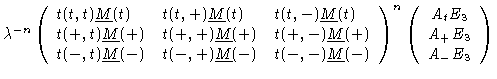$$\lambda^{-n} \left( {\begin{array}{lll} t(t,t)\underline{M}(t) & ... ...n \left( {\begin{array}{c} A_t E_3 \\ A_+ E_3 \\ A_- E_3 \end{array}} \right)$$ (1.37)

where E₃ is the 3-d unit matrix. In terms of direct products of matrices this reads

$$\langle \underline{M}(\varphi_i) \cdots \underline{M}(\varphi_{i+n-1}) \rangle = (B^T \otimes E_3) S^n (A \otimes E_3)$$ (1.38)

$$\lambda^{-1} \left( {\begin{array}{lll} t(t,t)\underline{M}(t) & ... ...ne{M}(-) & t(-,+)\underline{M}(-) & t(-,-)\underline{M}(-) \end{array}} \right)$$ S =

$$\lambda^{-1} \left( {\begin{array}{lll} t(t,t)E_3 & t(t,+)E_3 & t... ... \\ 0 & \underline{M}(+) & 0 \\ 0 & 0 & \underline{M}(-) \end{array}} \right)$$ =

$$\lambda^{-1} (T \otimes E_3) \Vert \underline{M} \Vert.$$ = (1.39)

Introducing everything into Eq. (1.35) we get

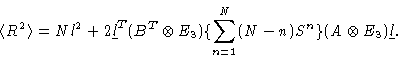$$\langle R^2 \rangle = N l^2 + 2 \underline{l}^T (B^T \otimes E_3) \{ \sum_{n=1}^N (N-n) S^n \} (A \otimes E_3) \underline{l}.$$ (1.40)

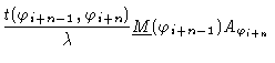
For infinitely long chains we can analytically sum, obtaining

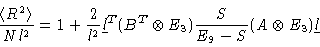$$\frac{\langle R^2 \rangle}{Nl^2} = 1 + \frac{2}{l^2} \underli... ...^T \otimes E_3) \frac{S}{E_9 -S} (A \otimes E_3) \underline{l}$$ (1.41)

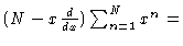
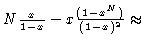
where E₉ is the 9-d unit matrix. In this derivation of Eq. (1.41) we have made use of $\sum_{n=1}^N (N-n)x^n =$ $(N-x \frac{d}{dx} ) \sum_{n=1}^N x^n =$ $N \frac{x}{1-x} - x \frac{(1-x^N)}{(1-x)^2} \approx$ $N \frac{x}{1-x}$ for large N.

Similar equations, but much more complicated, may be derived for $\langle R^{4}\rangle$. For these and other equations we refer to P.J. Flory, Statistical Mechanics of Chain Molecules .